Interpolating wavelets and their application to incremental signal
reconstruction from scattered data.
Learn how to build a wavelet tree such that approximation error locally only
depends on a local sample density.
Wavelet expansion is an efficient way to represent functions and operators.
In such an expansion, a function is decomposed into fluctuations at various
resolutions plus an averaged information at the coarsest resolution.
Their main advantage over traditional Fourier methods is their hability
to handle situations where the target signal contains discontinuities and
sharp spikes.
In this project we will take a closer look to interpolating wavelets and
their application to incremental signal reconstruction from scattered data.
We will build a wavelet tree such that approximation error locally only
depends on a local sample density.
1) Objective:
Approximate an unknown target function $f(x) = e^x\;cos(10x)\;cos(75x)$ on
$\Omega = [0,1]$ given $N$ consecutive (possibly noisy) uniformly distributed
samples $(x_i, f(x_i))$.
2) Choosing and generating scaling functions:
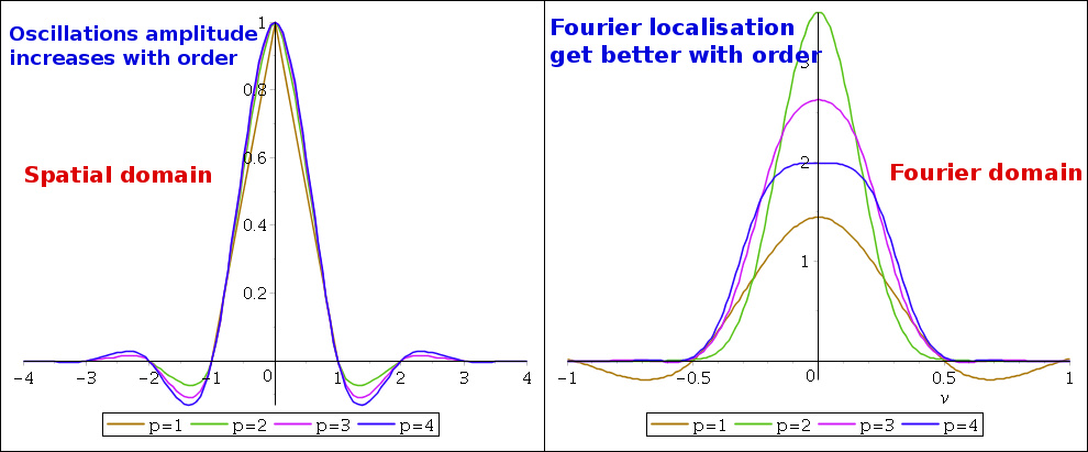
For this application we will use dyadic interpolating Deslauriers-Dubuc wavelets
up to a certain order $p$.
We can generate $\phi^k_p(x)$ at resolution $2^{-k}$ by recursively applying $k$ moving
Lagrange interpolation of order p to initial $\phi^0_p(x_i) = \delta_{i0}$ where
$x_i=i\;\;\forall i \in [[-2p+1, 2p+1]]$.
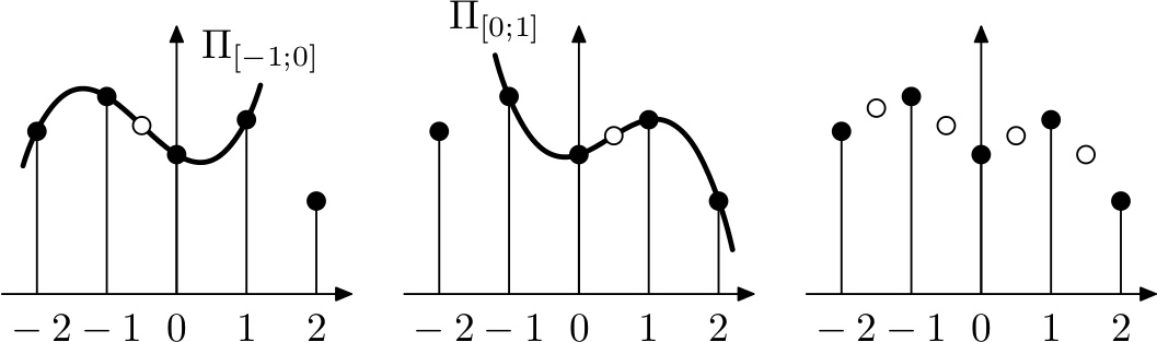
For each subinterval [$x_{k}, x_{k+1}]$ we generate a new
point $x_{k+1/2}$ by fitting a polynomial $\Pi_k(x)$ of degree $p$ to surrounding
points (not centered on interval at boundaries) and by evaluating $\Pi_k(x_{k+1/2})$.
The resulting scaling functions $\phi^p(x)$ are symmetric with support
$[-2p+1/2, 2p-1/2]$ and have $2p$ vanishing moments.
By defining the mother wavelet $\Psi^p(x)=\phi^p(2x-1)$ and the wavelet family
$\Psi^p_{jk} = \Psi^p(2^jx-k)$ we can define our wavelet basis at order $p$ by
$\mathcal{B}^p_0 = \{\Psi^p_{jk}\;|\;j=0 \textrm{ or } (j,k) \in \mathbb{N}^*
\times (2 \mathbb{Z} + 1)\}$.
As we want to apply approximation to the finite interval $\Omega = [0, 1]$, we would normally need
to construct explicit boundary wavelets as linear combinations of wavelets truncated at the boundary.
Here we will follow a simpler approach which is to take boundary filters of lower order.
Of course the new boundary-adapted basis $\mathcal{B}_1^p$ is not orthogonal and
we will need to solve a linear system to find the wavelet coefficients.